Introduction
This notebook presents a method to train embedding layer using Word2Vec Skip-Gram method on Wikipedia text8 dataset.
We are going to work with text8 dataset. It is 100MB of cleaned English Wikipedia text. $\text{10MB} = 10^8$ hence text8
Dataset:
- Large Text Compression Benchmark - About the test data - download file named text8.zip and unzip it.
References:
- Word2Vec Tutorial - The Skip-Gram Model - plain English tutorial on Skip-Grams
- Efficient Estimation of Word Representations in Vector Space - first skip-gram paper
- Distributed Representations of Words and Phrases and their Compositionality - follow up paper with improvements

Imports
import time
import math
import collections
import numpy as np
import matplotlib.pyplot as plt
import torch
import torch.nn as nn
import torch.optim as optim
import torch.nn.functional as F
device = torch.device("cuda:0" if torch.cuda.is_available() else "cpu")
Read Data
Dataset location
dataset_location = '/home/marcin/Datasets/wiki-text8/text8'
with open(dataset_location, 'r') as f:
    text = f.read()
print(text[:500])
Dataset is cleaned, it contains only lowercase letters and spaces
print(sorted(set(text)))
words_raw = text.split()
print(words_raw[:20])
print('Total words:', len(words_raw))
print('Unique words:', len(set(words_raw)))
Preprocess the Data
First we will look at word-count distribution
words_counter = collections.Counter(words_raw)
print('WORD : COUNT')
for w in list(words_counter)[:10]:
    print(w, ':', words_counter[w])
Lets plot word-counts on linear and logarithmic scales
sorted_all = np.array(sorted(list(words_counter.values()), reverse=True))
fig, [ax1, ax2] = plt.subplots(1, 2, figsize=[16,6])
ax1.plot(sorted_all); ax1.set_title('Word Counts (linear scale)')
ax2.plot(sorted_all); ax2.set_title('Word Counts (log scale)')
ax2.set_yscale('log')
This is extremely sharp distribution. Some words appear over 1 million times, while over 100k words appear only once.
Common Words
Lets have a look at the most common words.
words_counter.most_common()[:10]
We will deal with this later on using subsampling as described by Mikolov.
Rare Words
Lets look at some of of the uncommon words
words_counter.most_common()[-10:]
Words like 'metzanda' or 'metzunda' are so rare (first ever time I see these) we are not concerned about them when building our NLP system. We will subsequently drop all words that 5 or less times.
Create dictionaries
Tokenize words, but keep only ones that occur six or more times
i2w = {i : w for i, (w, c) in enumerate(words_counter.most_common()) if c > 5}
w2i = {w : i for i, w in i2w.items()}
print('Number of words after filter:', len(i2w))
Confirm both dictionaries check
for i in range(10):
    word = i2w[i]
    print(i, ':', word, ':', w2i[word])
Tokenize
words_tok = [w2i[w] for w in words_raw if w in w2i]
print('Number of words after removing uncommon:', len(words_tok))
This is our text, with uncommon words removed and converted to tokens:
print(words_tok[:100])
Subsampling
Equation from the paper, where $P(w_i)$ is probability to drop certain word, $f(w_i)$ is a frequency and $t$ is a parameter
Calculate probabilities
threshold = 1e-5

tokens_counter = collections.Counter(words_tok)    # token : num_occurances

prob_drop = {}
for tok, count in tokens_counter.items():
    word_freq = count / len(words_tok)
    prob_drop[tok] = 1 - math.sqrt(threshold / word_freq)
Print probabilities for some words, note that for frequent words like 'the' drop probability is quite high while for uncommon words it is actually negative (meaning don't ever drop)
print('word        occurances     p_drop')
for word in ['the', 'at', 'dog', 'cat', 'extravagant', 'sustaining']:
    token = w2i[word]
    print(f'{word:11}    '
          f'{tokens_counter[token]:7}     '
          f'{prob_drop[token]: .2f}')
Drop words according to probability (we could do this on per-batch basis)
words_fin = [tok for tok in words_tok if np.random.rand() > prob_drop[tok] ]
Generate Training Dataset

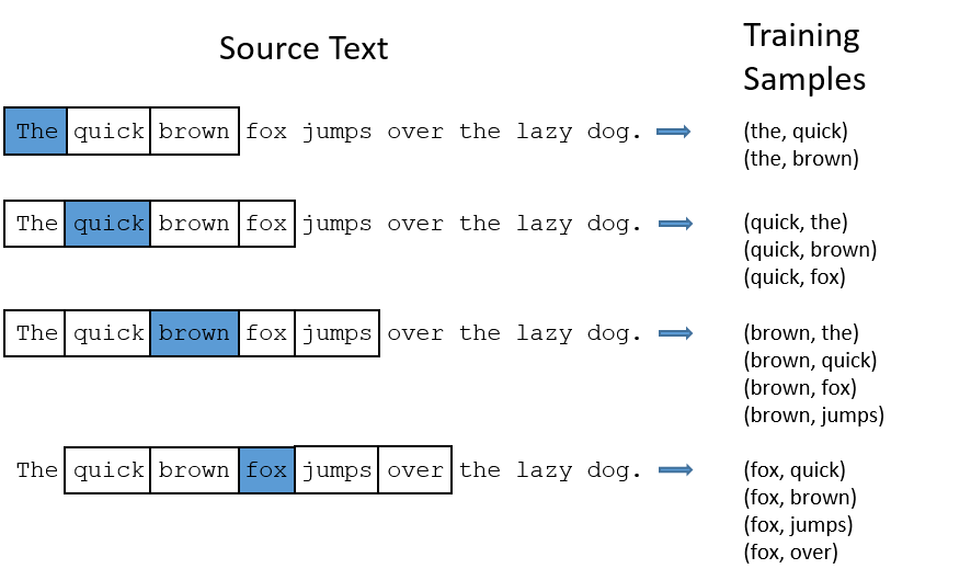
For each word sample the surrounding context of $R$ words on each side. To reflect the fact that more distant words are less relevant we pick $R$ as a random integer in range $[1:\text{max_window}]$ This could also be done on per-batch basis
max_window = 5

data_x, data_y = [], []

for i, tok in enumerate(words_fin):
    R = np.random.randint(1, max_window+1)
    start = max(i - R, 0)
    stop = i + R
    targets = words_fin[start:i] + words_fin[i+1:stop+1]

    data_x.extend([tok] * len(targets))
    data_y.extend(targets)
Show sample data
print('Original:', words_fin[:10])
print('Inputs: ', data_x[:10])
print('Targets:', data_y[:10])
Convert to tensors
train_x = torch.tensor(data_x).to(device)
train_y = torch.tensor(data_y).to(device)
Skip-Gram Model
class SkipGram(nn.Module):
    def __init__(self, n_vocab, n_embed):
        super(SkipGram, self).__init__()
        self.embed = nn.Embedding(num_embeddings=n_vocab, embedding_dim=n_embed)
        self.fc = nn.Linear(n_embed, n_vocab)

    def forward(self, x):
        x = self.embed(x)
        return self.fc(x)
n_vocab = len(w2i)  # size of vocabulary
n_embed = 300       # size of embedding dimension
model = SkipGram(n_vocab, n_embed)
model.to(device)
criterion = nn.CrossEntropyLoss()
optimizer = optim.Adam(model.parameters(), lr=0.003)
def get_most_similar(model, test_words, topk):
    result = {}
    with torch.no_grad():
        for word in test_words:
            tok = w2i[word]
            x = torch.tensor([tok]).to(device)
            x_embed = model.embed(x)
            cos_sim = F.cosine_similarity(x_embed, model.embed.weight)
            _, indices = cos_sim.topk(topk+1)  # +1 because self is always most similar
            similar_words = [i2w[tok.item()] for tok in indices]
            result[word] = similar_words[1:]

    return result
n_batch = 3072
nb_epochs = 1

trace = {'loss': []}  # per iteration

iteration = 0
for epoch in range(1):

    time_start = time.time()

    #
    #   Train Model
    #
    model.train()
    for i in range(0, len(train_x), n_batch):

        # Pick mini-batch (over seqence dimension)
        inputs = train_x[i:i+n_batch]    # [n_batch]
        targets = train_y[i:i+n_batch]   # [n_batch]

        # Optimize
        optimizer.zero_grad()
        outputs = model(inputs)  # logits
        loss = criterion(outputs, targets)
        loss.backward()
        optimizer.step()

        # Record
        trace['loss'].append( loss.item() )

        if i % (100*n_batch) == 0:
            percent_complete = i * 100 / len(train_x)
            time_delta = time.time() - time_start
            print(f'Epoch: {epoch:3} ({percent_complete:.0f}%)     '
                f'Loss: {loss:.4f}     Time: {time_delta:.2f}s')

            test_words = ['king', 'rock', 'dog', 'jump', 'five', 'http']
            res_dict = get_most_similar(model, test_words, topk=5)
            for word, similar in res_dict.items():
                print(f'{word:<6}:', ' '.join(similar))
            print('----------')

            time_start = time.time()
After one epoch it picks up numbers and web domains. It needs couple more epochs at lest.