$$ \huge{\underline{\textbf{ Simple Bandit Algorithm }}} $$

In [1]:
def simple_bandit(env, nb, eps):
    Q = np.zeros(env.size)
    N = np.zeros(env.size)

    for _ in range(nb):
        A = argmax_rand(Q) if np.random.rand() > eps else np.random.randint(env.size)
        R = env.step(A)
        N[A] += 1
        Q[A] += (1/N[A]) * (R - Q[A])

    return Q
Helper functions:
In [2]:
def argmax_rand(arr):
    # break ties randomly, np.argmax() always picks first max
    return np.random.choice(np.flatnonzero(arr == arr.max()))
 |
 |
Experiment Setup
In [3]:
import numpy as np
import matplotlib.pyplot as plt
Environment
In [4]:
class BanditEnv:
    def __init__(self):
        """10-armed testbed, see chapter 2.3"""
        self.size = 10                                        # 10 arms
        self.means = np.array([0.25, -0.75, 1.5, 0.5, 1.25,   # eyeball fig 2.1
                               -1.5, -0.25, -1, 0.75, -0.5])
    def step(self, action):
        return np.random.normal(loc=self.means[action])
Add history logging
In [5]:
def simple_bandit(env, nb, eps):
    hist_A = []
    hist_R = []

    Q = np.zeros(env.size)
    N = np.zeros(env.size)

    for _ in range(nb):
        A = argmax_rand(Q) if np.random.rand() > eps else np.random.randint(env.size)
        R = env.step(A)
        N[A] += 1
        Q[A] += (1/N[A]) * (R - Q[A])

        hist_A.append(A)
        hist_R.append(R)

    return Q, np.array(hist_A), np.array(hist_R)
Recreate Figure 2.1
In [6]:
env = BanditEnv()

fig = plt.figure()
ax = fig.add_subplot(111)
parts = ax.violinplot(np.random.randn(2000,10) + env.means,
                      showmeans=True, showextrema=False)
for pc in parts['bodies']: pc.set_facecolor('gray')
parts['cmeans'].set_color('gray')
ax.plot([0,10],[0,0], color='gray', linestyle='--')
ax.set_ylim([-4, 4])
ax.set_xlabel("Action"); ax.set_ylabel("Reward Distribution")
plt.tight_layout()
plt.savefig('assets/fig_0201.png')
plt.show()

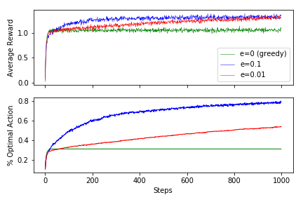
Recreate Figure 2.2
Generate raw data, this may take a while
In [7]:
env = BanditEnv()

runs_ep0_A, runs_ep0_R = [], []      # eps=0, greedy
runs_ep01_A, runs_ep01_R = [], []    # eps=0.1
runs_ep001_A, runs_ep001_R = [], []  # eps=0.01

print('v' + ' '*18 + 'v')  # poor man tqdm
for i in range(2000):
    _, hist_A, hist_R = simple_bandit(env, nb=1000, eps=0)
    _, runs_ep0_A.append(hist_A); runs_ep0_R.append(hist_R);

    _, hist_A, hist_R = simple_bandit(env, nb=1000, eps=0.1)
    _, runs_ep01_A.append(hist_A); runs_ep01_R.append(hist_R);

    _, hist_A, hist_R = simple_bandit(env, nb=1000, eps=0.01)
    _, runs_ep001_A.append(hist_A); runs_ep001_R.append(hist_R);

    if i % 100 == 0: print('.', end='')

runs_ep0_A, runs_ep0_R = np.array(runs_ep0_A), np.array(runs_ep0_R)
runs_ep01_A, runs_ep01_R = np.array(runs_ep01_A), np.array(runs_ep01_R)
runs_ep001_A, runs_ep001_R = np.array(runs_ep001_A), np.array(runs_ep001_R)
Calc average reward and % optimal action
In [8]:
# Calc average reward
avg_ep0_R = np.average(runs_ep0_R, axis=0)
avg_ep01_R = np.average(runs_ep01_R, axis=0)
avg_ep001_R = np.average(runs_ep001_R, axis=0)

# Calc "% optimal action"
max_A = np.argmax(env.means)
opt_ep0_A = np.average(runs_ep0_A==max_A, axis=0)
opt_ep01_A = np.average(runs_ep01_A==max_A, axis=0)
opt_ep001_A = np.average(runs_ep001_A==max_A, axis=0)
Pretty plot
In [9]:
fig = plt.figure()
ax = fig.add_subplot(211)
ax.plot(avg_ep0_R,   linewidth=0.5, color='green', label='e=0 (greedy)')
ax.plot(avg_ep01_R,  linewidth=0.5, color='blue',  label='e=0.1')
ax.plot(avg_ep001_R, linewidth=0.5, color='red',   label='e=0.01')
ax.set_ylabel('Average Reward')
ax.xaxis.set_ticklabels([])
ax.legend()

ax = fig.add_subplot(212)
ax.plot(opt_ep0_A,   linewidth=1., color='green', label='e=0 (greedy)')
ax.plot(opt_ep01_A,  linewidth=1., color='blue',  label='e=0.1')
ax.plot(opt_ep001_A, linewidth=1., color='red',   label='e=0.01')
ax.set_xlabel('Steps'); ax.set_ylabel('% Optimal Action')

plt.tight_layout()

plt.savefig('assets/fig_0202.png')
plt.show()

Other Tests
Confirm Q-Values are estimated correctly
In [10]:
env = BanditEnv()

Q, _, _ = simple_bandit(env, nb=10000, eps=0.5)

print('True:   ', np.round(env.means, 3))
print('Q:      ', np.round(Q, 3))
print('True - Q', np.round(env.means-Q, 3))

plt.scatter(range(env.size), env.means, color='blue', marker='o', label='true')
plt.scatter(range(env.size), Q, color='red', marker='x', label='Q')
plt.legend();
