$$ \huge{\underline{\textbf{ Monte Carlo ES Control }}} $$

In [1]:
def monte_carlo_ES_control(env, ep, gamma):
    """Monte Carlo ES Control
    Params:
        env - environment
        ep - number of episodes to run
        gamma - discount factor
    """

    pi = defaultdict(int)        # default action: 0
    Q = defaultdict(float)       # default Q value: 0
    Returns = defaultdict(list)  # dict of lists

    for _ in range(ep):
        S0, A0 = env.sample_state_action()
        traj, T = generate_episode_ES(env, pi, S0, A0)
        G = 0
        for t in range(T-1,-1,-1):
            St, _, _, At = traj[t]      # (st, rew, done, act)
            _, Rt_1, _, _ = traj[t+1]

            G = gamma * G + Rt_1

            if not (St, At) in [(traj[i][0], traj[i][3]) for i in range(0, t)]:
                Returns[(St, At)].append(G)
                Q[(St, At)] = np.average(Returns[(St, At)])
                pi[St] = np.argmax([Q[St,a] for a in range(env.nb_actions)])

    return Q, pi
Helper functions:
In [2]:
def generate_episode_ES(env, pi, S0, A0):
    """Generete one complete episode.

    Returns:
        trajectory: list of tuples [(st, rew, done, act), (...), (...)],
                    where St can be e.g tuple of ints or anything really
        T: index of terminal state, NOT length of trajectory
    """
    trajectory = []
    done = True
    while True:
        # === time step starts here ===
        if done:
            St, Rt, done    = env.reset_es(S0), None, False
            At = A0
        else:
            St, Rt, done, _ = env.step(At)
            At = pi[St]
        trajectory.append((St, Rt, done, At))
        if done:  break
        # === time step ends here ===
    return trajectory, len(trajectory)-1
 |
Solve Blackjack
In [3]:
import numpy as np
import matplotlib.pyplot as plt
from collections import defaultdict
from mpl_toolkits.mplot3d import axes3d
import gym
Extend OpenAI Gym Blackjack-v0 to allow exploring starts
In [4]:
class BlackjackES():
    def __init__(self):
        self._env = gym.make('Blackjack-v0')
        self.nb_actions = 2

    def sample_state_action(self):
        """Sample and return valid state & action for exp. starts"""
        player_sum = np.random.randint(12, 22)
        dealer_shows = np.random.randint(1, 11)
        has_ace = np.random.randint(0, 2)
        state = (player_sum, dealer_shows, bool(has_ace))
        action = np.random.randint(0, 2)
        return state, action

    def reset_es(self, init_state):
        """Start game from given state"""
        player_sum, dealer_shows, has_ace = init_state
        assert player_sum in range(12, 22)
        assert dealer_shows in range(1, 11)
        assert isinstance(has_ace, bool)

        self._env.reset()  # reset OpenAI env

        # draw second card for the dealer
        # according to original probabilities
        dealer_hides = np.random.choice([1, 2, 3, 4, 5, 6, 7,
                                         8, 9, 10, 10, 10, 10])

        # override dealer hand
        self._env.dealer = [dealer_shows, dealer_hides]

        # pick cards for player to match player_sum and has_ace
        if has_ace:
            player_hand = [player_sum-11, 1]
        else:
            if player_sum == 21:  player_hand = [10, 9, 2]
            else:                 player_hand = [player_sum-10, 10]

        # override player hand
        self._env.player = player_hand

        # force re-evaluate observation with new hands
        obs = self._env._get_obs()
        assert obs == init_state
        return obs

    def step(self, action):
        return self._env.step(action)
Create environment
In [5]:
env = BlackjackES()
Ploting
In [6]:
from helpers_0503 import plot_blackjack
Solve Blackjack
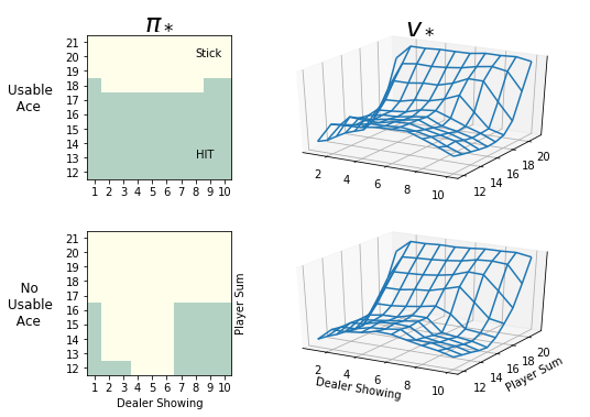
- result is only a quick approximation, very unlikely to match the book figure 5.2 exactly
- but with (many) more samples, this will converge to same policy as in the book
In [7]:
Q, pi = monte_carlo_ES_control(env, ep=250000, gamma=1.0) # approx 1 min to run
In [8]:
plot_blackjack(Q, pi)

Recreate Figure 5.2
In blackjack as presented in the book some states are very difficult to evaluate correctly, because Q-values for hit and stick is almost identical. It takes huge amount of samples to evaluate these states correctly.
First, we will have to modify original algorithm slightly, changes include:
- new parameters:
- add callback parameter - user function called every training episode
- add resume_dicts param - this is so we can pick up training from where we left
- add focus_S0 param - this overrides random initial state selection with single state
- Returns now stores sum of Q-Values, not list of all Q-Values - important speed improvement for longer runs!
- C dict stores number of vistis for each state
- We skip step to check if this is first-visit to state St - this effectively changes algorithm to Every-Visit MC.
In [9]:
def monte_carlo_ES_control_ext(env, ep, gamma, callback=None, resume_dicts=None, focus_S0=None):
    """Monte Carlo ES Control
    Params:
        env - environment
        ep - number of episodes to run
        gamma - discount factor
    """
    if resume_dicts is None:
        pi = defaultdict(int)         # this is same as before
        C = defaultdict(int)          # Change! count number of visits!
        Returns = defaultdict(float)  # Change! this is SUM now
        Q = defaultdict(float)        # this didn't change either
    else:
        pi, C, Returns, Q = resume_dicts

    for e in range(ep):
        S0, A0 = env.sample_state_action()
        if focus_S0 is not None: S0 = focus_S0

        traj, T = generate_episode_ES(env, pi, S0, A0)
        G = 0
        for t in range(T-1,-1,-1):
            St, _, _, At = traj[t]      # (st, rew, done, act)
            _, Rt_1, _, _ = traj[t+1]

            G = gamma * G + Rt_1

            # Change to every-visit MC to save computation
            C[(St, At)] += 1
            Returns[(St, At)] += G
            Q[(St, At)] = Returns[(St, At)] / C[(St, At)]
            pi[St] = np.argmax([Q[St,a] for a in range(env.nb_actions)])

        if callback is not None:
            callback(e, Q)

    return Q, pi, (pi, C, Returns, Q)
Define callback functions
- trace is a long list np.arrays - each array is 4d with dims: [player_sum, dealer_card, has_ace, action]
In [10]:
trace = []         # track Q-Values during training, don't forget to clear between runs!

def convert_to_sum(Q):
    # convert dict to 4d array
    # dims are: [player_sum, dealer_card, has_ace, action]
    res = np.zeros([10, 10, 2, 2])
    for ps in range(12,22):
        for dc in range(1, 11):
            for ha in [0, 1]:
                for act in [0, 1]:
                    res[ps-12, dc-1, ha, act] = Q[(ps, dc, bool(ha)), act]
    return res

def callback(ep, Q):
    if ep % 1000 == 0:
        trace.append(convert_to_sum(Q))  # append Q-Array (not dict)
Import new fancy plotting function
In [11]:
from helpers_0503 import plot_Q_trace
Start new training session, this time with trace
In [12]:
# Option 1 - START NEW TRAINING
trace = []
Q, pi, resume = monte_carlo_ES_control_ext(env, ep=1000000, gamma=1.0, callback=callback)

# Option 2 - CONTINUE
# run this as many times as required until convergence
# Q, pi, resume = monte_carlo_ES_control_ext(env, ep=1000000, gamma=1.0, callback=callback, resume_dicts=resume)
Investigate progress
In [13]:
print('Training episodes so far: ', len(trace)*1000)
plot_blackjack(Q, pi)
# plot_Q_trace(trace, has_ace=0)                   # plot everything
plot_Q_trace(trace, has_ace=0, start_at=-1000)     # plot last 1000000 episodes


Above plot shows how Q-Values develop over time, couple notes:
- $\color{blue}{\text{"Stick" is blue}}$, $\color{red}{\text{"HIT" is red}}$
- this plot corresponds in layout to "No Usable Ace" policy plot
- each small plot is history of Q-Values for that state
- for some states Q-Values for Stick/Hit diverge immediately and stay apart
- for some states, especially some states in the row Player Sum == 12, Q-Values are very close together
Save the plot when done
In [14]:
# plot_blackjack(Q, pi, save_path='assets/fig_0503.png')
Timing Tests
In [15]:
%timeit -r1 monte_carlo_ES_control(env, ep=10000, gamma=1.0)
%timeit -r1 monte_carlo_ES_control_ext(env, ep=10000, gamma=1.0)
In [16]:
%timeit -r1 monte_carlo_ES_control(env, ep=100000, gamma=1.0)
%timeit -r1 monte_carlo_ES_control_ext(env, ep=100000, gamma=1.0)
In [17]:
%timeit -r1 monte_carlo_ES_control(env, ep=1000000, gamma=1.0)
%timeit -r1 monte_carlo_ES_control_ext(env, ep=1000000, gamma=1.0)