$$ \huge{\underline{\textbf{ Gradient Monte Carlo }}} $$
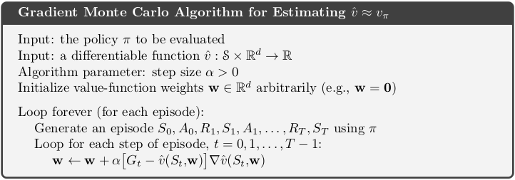
Implementation below matches the box exactly, but is for educational purposes only. See notes.
Notes:
- function approximator should be implemented as independent object - passing vector w around is impractical in actual program
- I'm not sure why time step loop iterates foward (t=0,1..,T-1) instead of backwards (t=T-1,T-2,..,0), like we did in previous chapters (backward implementation is more efficient and avoids ackward Gt computation every time step)
- algorithm in the box is for undiscounted case and thus omnits $\gamma$ parameter
- For alternative implementation, which fixes above issues, see further below.
def gradient_MC(env, policy, ep, alpha, init_w, v_hat, grad_v_hat):
    """Gradient Monte Carlo Algorithm

    Params:
        env        - environment
        policy     - function in a form: policy(state)->action
        ep         - number of episodes to run
        alpha      - step size (0..1]
        init_w     - function if form init_w() -> weights
        v_hat      - function in form v_hat(state, weights) -> float
        grad_v_hat - function in form grad_v_hat(state, weights) -> delta_weights
    """
    w = init_w()

    for _ in range(ep):
        traj, T = generate_episode(env, policy)
        for t in range(T):
            St, _, _, _ = traj[t]                            # (st, rew, done, act)
            Gt = sum([traj[i][1] for i in range(t+1, T+1)])  # <- this is inefficient
            w = w + alpha * (Gt - v_hat(St, w)) * grad_v_hat(St, w)

    return w
Helper functions:
def init_w():
    return np.zeros(10)      # weights for 10 groups

def v_hat(St, w):
    group = (St-1) // 100    # [1-100, 101-200, ..., 901-1000] -> [0, 1, ..., 9]
    return w[group]

def grad_v_hat(St, w):
    grad = np.zeros_like(w)
    grad[(St-1)//100] = 1
    return grad
def generate_episode(env, policy):
    """Generete one complete episode.

    Returns:
        trajectory: list of tuples [(st, rew, done, act), (...), (...)],
                    where St can be e.g tuple of ints or anything really
        T: index of terminal state, NOT length of trajectory
    """
    trajectory = []
    done = True
    while True:
        # === time step starts here ===
        if done:  St, Rt, done = env.reset(), None, False
        else:     St, Rt, done = env.step(At)
        At = policy(St)
        trajectory.append((St, Rt, done, At))
        if done:  break
        # === time step ends here ===
    return trajectory, len(trajectory)-1
 |
Alternative Implementation
This section is very important, it is heavily built uppon in following chapters. We will reuse this implementation a lot later on. It's best to get good understanding right here, including both options 1 and 2 in the AggregateFunctApprox.
This implementation includes following features as compared with original implementation above:
- function approximator is now a trainable black-box object - can be tabular, linear, neural-net
- added discount paramter $\gamma$
- time-step loop now goes backward for efficiency
def gradient_MC_fix(env, policy, ep, gamma, model):
    """Gradient Monte Carlo Algorithm

    Params:
        env    - environment
        policy - function in a form: policy(state)->action
        ep     - number of episodes to run
        gamma  - discount factor [0..1]
        model  - function approximator, already initialised, with method:
                     train(state, target) -> None
    """
    for _ in range(ep):
        traj, T = generate_episode(env, policy)
        Gt = 0
        for t in range(T-1,-1,-1):
            St, _, _, _ = traj[t]      # (st, rew, done, act)
            _, Rt_1, _, _ = traj[t+1]

            Gt = gamma * Gt + Rt_1
            model.train(St, Gt)
Aggregate Function Approximator
class AggregateFunctApprox():
    """Very simple function approximator"""
    def __init__(self, learn_rate, nb_groups, group_size):
        self._lr = learn_rate
        self._group_size = group_size
        self._w = np.zeros(nb_groups)  # weights

    def evaluate(self, state):
        # Option 1:
        group = (state-1) // self._group_size      # [1-100, ..., 901-1000] -> [0, ..., 9]
        return self._w[group]                      # return corresponding value

        # Option 2:
        # Implement as a special case of linear combination of features
#         group = (state-1) // self._group_size    # [1-100, ..., 901-1000] -> [0, ..., 9]
#         x = np.zeros_like(self._w)
#         x[group] = 1                             # one-hot encoded feature vector [0, 1, 0]
#         return x @ self._w                       # linear combination, i.e. dot product

    def train(self, state, target):
        # Option 1:
        # Because grad_v_hat is a one-hot vector, we can optimize:
        group = (state-1) // self._group_size
        self._w[group] += self._lr * (target - self._w[group])  # update only one weight,
                                                                # standard MC update!

        # Option 2:
#         group = (state-1) // self._group_size
#         x = np.zeros_like(self._w)
#         x[group] = 1                              # one-hot feature vector
#         grad = x                                  # grad. of lin. comb. is just x
Evaluate Example 9.1
import numpy as np
import matplotlib.pyplot as plt
from collections import defaultdict
Define environment
- V_approx values were picked by trial-and-error, they ignore both nonlinearity and terminal states (which should equal zero)
class LinearEnv:
    """
    State nb:   [   0       1   ...   499   500   501   ...   1000    1001  ]
    State type: [terminal   .   ...    .   start   .    ...     .   terminal]
    """
    V_approx = np.arange(-1001, 1001, 2) / 1000.0  # ignore nonlinearity at terminal states

    def __init__(self):
        self.reset()

    def reset(self):
        self._state = 500
        self._done = False
        return self._state

    def step(self, action):
        if self._done: raise ValueError('Episode has terminated')

        if action == 0:   self._state -= np.random.randint(1, 101)  # step left
        elif action == 1: self._state += np.random.randint(1, 101)  # step right
        else: raise ValueError('Invalid action')

        self._state = np.clip(self._state, 0, 1001)  # clip to 0..1001
        if self._state in [0, 1001]:                 # both 0 and 1001 are terminal
            self._done = True

        if self._state == 0:
            return self._state, -1, self._done       # state, rew, done
        elif self._state == 1001:
            return self._state, 1, self._done
        else:
            return self._state, 0, self._done
Plotting
def plot_linear(V, env, freq=None, saveimg=None):
    fig = plt.figure()
    ax = fig.add_subplot(111)
    # Note, state 0 is terminal, so we exclude it
    ax.plot(range(1,1001), env.V_approx[1:], color='red', linewidth=0.8, label='"True" value')
    ax.plot(range(1,1001), V[1:], color='blue', linewidth=0.8, label='Approx. MC value')
    ax.set_xlabel('State')
    ax.set_ylabel('Value Scale')
    ax.legend()

    if freq is not None:
        mu = np.zeros(len(V))       # convert to array, V has same len as freq
        for st in range(len(V)):
            mu[st] = freq[st]
        ax2 = ax.twinx()
        # again, exclude terminal state 0
        ax2.bar(range(1,1001), mu[1:], color='gray', width=5, label='State Distr.')
        ax2.set_ylabel('Distribution Scale')
        ax2.legend(loc='right', bbox_to_anchor=(1.0, 0.2))

    plt.tight_layout()
    if saveimg is not None:
        plt.savefig(saveimg)
    plt.show()
Create environment
env = LinearEnv()
Random policy
def policy(st):
    return np.random.choice([0, 1])
Solve with original algorithm
weights = gradient_MC(env, policy, ep=10000, alpha=0.0003,
                      init_w=init_w, v_hat=v_hat, grad_v_hat=grad_v_hat)
V = [v_hat(st, weights) for st in range(1001)]
plot_linear(V, env)

Solve with proper function approximator
model = AggregateFunctApprox(learn_rate=0.0003, nb_groups=10, group_size=100)
gradient_MC_fix(env, policy, ep=5000, gamma=1.0, model=model)
V = [model.evaluate(st) for st in range(1001)]
plot_linear(V, env)

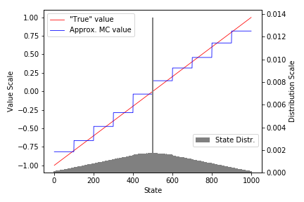
Recreate Figure 9.1
We need to track frequency of visit to each state, let's modify our algorithm slightly. Changes are marked with arrows.
def gradient_MC_track_freq(env, policy, ep, gamma, model):
    count = defaultdict(float)  # <- how many times state visited
    total = 0                   # <- total state visits to all states

    for _ in range(ep):
        traj, T = generate_episode(env, policy)
        Gt = 0
        for t in range(T-1,-1,-1):
            St, _, _, _ = traj[t]      # (st, rew, done, act)
            _, Rt_1, _, _ = traj[t+1]

            count[St] += 1
            total += 1

            Gt = gamma * Gt + Rt_1
            model.train(St, Gt)

    for key, val in count.items():  # <- calc. frequency
        count[key] = val / total

    return count                    # <- return freq.
Solve.
- In the book alg. is run for 100k episodes, alpha=2e-5. Here we run for 10k episodes alpha=1e-4 to save time.
model = AggregateFunctApprox(learn_rate=0.00001, nb_groups=10, group_size=100)  # +10min?
freq = gradient_MC_track_freq(env, policy, ep=100000, gamma=1.0, model=model)
Plot
V = [model.evaluate(st) for st in range(1001)]
plot_linear(V, env, freq=freq, saveimg=None)  # 'assets/fig_0901.png'
