$$ \huge{\underline{\textbf{ Linear Models }}} $$
$$ \large{\textbf{ Polynomial and Fourier Bases }} $$
We are going to use Gradient MC algorithm from chapter 9.3 as a learning algorithm. Before continuing you should familiarise yourself properly with chapter 9.3. We will use the "fixed" version of Gradient MC, repeated here for reference.
One notable difference is that this version takes callback and trace arguments, so we can log results after each episode. This is used to reproduce figures in the book.
def gradient_MC(env, policy, ep, gamma, model, callback=None, trace=None):
    """Gradient Monte Carlo Algorithm

    Params:
        env    - environment
        policy - function in a form: policy(state)->action
        ep     - number of episodes to run
        gamma  - discount factor [0..1]
        model  - function approximator, already initialised, with method:
                     train(state, target) -> None
        callback - function in a form: callback(episode, model, trace) -> None
        trace  - passed to callback, so it can log data into it
    """
    for e_ in range(ep):
        traj, T = generate_episode(env, policy)
        Gt = 0
        for t in range(T-1,-1,-1):
            St, _, _, _ = traj[t]      # (st, rew, done, act)
            _, Rt_1, _, _ = traj[t+1]

            Gt = gamma * Gt + Rt_1
            model.train(St, Gt)

        if callback is not None:
            callback(e_, model, trace)
def generate_episode(env, policy):
    """Generete one complete episode.

    Returns:
        trajectory: list of tuples [(st, rew, done, act), (...), (...)],
                    where St can be e.g tuple of ints or anything really
        T: index of terminal state, NOT length of trajectory
    """
    trajectory = []
    done = True
    while True:
        # === time step starts here ===
        if done:  St, Rt, done = env.reset(), None, False
        else:     St, Rt, done = env.step(At)
        At = policy(St)
        trajectory.append((St, Rt, done, At))
        if done:  break
        # === time step ends here ===
    return trajectory, len(trajectory)-1
 |
Environment Setup
All environment and plotting code is exactly the same as in chapter 9.3. All the code is available here: helpers_0905.py
import numpy as np
import matplotlib.pyplot as plt
from helpers_0905 import LinearEnv, plot_linear
env = LinearEnv()
def policy(st):
    return np.random.choice([0, 1])
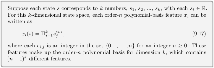
Polynomial Basis
In chapter 9.3 we approximated state value function by grouping 1000 states into 10 groups, each group with its own value. Here we will implement drop-in replacement for that approximator that will fit polynomial instead. Actually, as we will soon see, all approximators in this chapter are compatible drop-in replacements.
Box from the book as reference.
class PolynomialFuncApprox():
    """Polynomial function approximator"""
    def __init__(self, learn_rate, order, nb_states):
        self._lr = learn_rate
        self._order = order
        self._nb_states = nb_states
        self._w = np.zeros(order+1)                    # weights

    def reset(self):
        self._w = np.zeros(self._order+1)

    def evaluate(self, state):
        st01 = state / self._nb_states                 # map to 0..1
        x = np.power(st01, range(self._order+1))       # x = [st**0, st**1, ..., st**order]
        return x @ self._w                             # linear combination, i.e. dot product

    def train(self, state, target):
        st01 = state / self._nb_states                 # map to 0..1
        x = np.power(st01, range(self._order+1))       # x = [st**0, st**1, ..., st**order]
        grad = x                                       # grad. of lin. comb. is input x

        v_hat = self.evaluate(state)
        self._w += self._lr * (target - v_hat) * grad  # Gradient MC update, see chapt. 9.3
Polynomial Basis Test
model = PolynomialFuncApprox(learn_rate=0.0001, order=5, nb_states=1000)
gradient_MC(env, policy, ep=1000, gamma=1.0, model=model)
V = [model.evaluate(st) for st in range(1001)]
plot_linear(V, env)

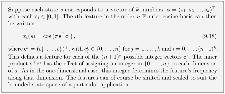
Fourier Basis
class FourierFuncApprox():
    """Polynomial function approximator"""
    def __init__(self, learn_rate, order, nb_states):
        self._lr = learn_rate
        self._order = order
        self._nb_states = nb_states
        self._w = np.zeros(order+1)                    # weights

    def reset(self):
        self._w = np.zeros(self._order+1)

    def evaluate(self, state):
        st01 = state / self._nb_states                 # map to 0..1
        c_i = np.arange(self._order+1)
        x = np.cos(np.pi * st01 * c_i)                 # x = [cos(pi*st*0), cos(pi*st*1), ...]
        return x @ self._w                             # linear combination, i.e. dot product


    def train(self, state, target):
        st01 = state / self._nb_states                 # map to 0..1
        c_i = np.arange(self._order+1)
        x = np.cos(np.pi * st01 * c_i)                 # x = [cos(pi*st*0), cos(pi*st*1), ...]
        grad = x                                       # grad. of lin. comb. is just x

        v_hat = self.evaluate(state)
        self._w += self._lr * (target - v_hat) * grad  # Gradient MC update, see chapt. 9.3
Fourier Basis Test
model = FourierFuncApprox(learn_rate=0.0001, order=5, nb_states=1000)
gradient_MC(env, policy, ep=1000, gamma=1.0, model=model)
V = [model.evaluate(st) for st in range(1001)]
plot_linear(V, env)

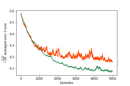
Recreate Figure 9.5
Callback is called by gradient_MC every single timestep:
- compute V for all states
- compute Root Mean Squared Error (skip terminal state 0, state 1001 is out of boundry)
- append to rmse list
def callback(episode, model, trace):
    """Called from gradient_MC after every episode.

    Params:
        episode [int] - episode number
        model [obj]   - function approximator
        trace [list]  - list to write results to"""
    V = np.array([model.evaluate(st) for st in range(1001)])                   # arr of float
    err = np.sqrt(np.mean(np.power((np.array(V[1:]) - env.V_approx[1:]), 2)))  # float
    trace.append(err)
Define experiment
def experiment(runs, env, policy, ep, gamma, model, callback):
    results = []  # dims: [nb_runs, nb_episodes]
    for r in range(runs):
        trace = []  # dim: [nb_episodes]
        model.reset()
        gradient_MC(env, policy, ep, gamma, model, callback=callback, trace=trace)
        results.append(trace)
    return np.average(results, axis=0)
Compute RMSE for polynomial approximator. This may take 5+ minutes.
model = PolynomialFuncApprox(learn_rate=0.0001, order=5, nb_states=1000)
poly_order_5 = experiment(3, env, policy, ep=5000, gamma=1.0, model=model, callback=callback)
And the Fourier approximator. This may take 5+ minutes.
model = FourierFuncApprox(learn_rate=0.00005, order=5, nb_states=1000)
fourier_order_5 = experiment(3, env, policy, ep=5000, gamma=1.0, model=model, callback=callback)
Plot results
fig = plt.figure()
ax = fig.add_subplot(111)
ax.plot(poly_order_5, color='orangered', label='Polynomial Basis (order=5)')
ax.plot(fourier_order_5, color='seagreen', label='Fourier Basis (order=5)')
ax.set_ylabel('$\sqrt{\overline{VE}}$ averaged over 3 runs')
ax.set_xlabel('Episodes')
# plt.savefig('assets/fig_0905.png')
ax.legend()
plt.show()
