$$ \Huge{\underline{\mathbf{ Dynamic \ Programming }}} $$
Introduction
Implementation of algorithms presented in Lecture 3 of UCL RL course by David Silver.
Contents:
- Intro
- Introduction - this section
- Frozen Lake - environment
- Algorithms
- Iterative Policy Evaluation - matrix form
- Policy Iteration - matrix form
- Value Iteration - loopy form
Notes:
- As OpenAI gym doesn't have environment corresponding to gridworld used in lectures. We use FrozenLake-v0 instead
Sources:
- UCL Course on RL: http://www0.cs.ucl.ac.uk/staff/d.silver/web/Teaching.html
- Lecture 3 pdf: http://www0.cs.ucl.ac.uk/staff/d.silver/web/Teaching_files/DP.pdf
- Lecture 3 vid: https://www.youtube.com/watch?v=Nd1-UUMVfz4
Imports:
import numpy as np
import gym
np.set_printoptions(linewidth=115)  # nice printing of large arrays

# Initialise variables used through script
env = gym.make('FrozenLake-v0')
nb_states = env.env.nS        # number of possible states
nb_actions = env.env.nA       # number of actions from each state
Frozen Lake
Documentation for FrozenLake-v0: https://gym.openai.com/envs/FrozenLake-v0/
Frozen Lake is 4x4 grid:
 Note on actions:
- environment is 'slippery' - choosing to go 'North' will result with 1/3 probability of moving West/North/East each.
- external walls are 'bouncy' - if action would result in falling off the grid, agent remains in current state instead
Let's make an environment
env = gym.make('FrozenLake-v0')
env.reset()
env.render()
Save number of states and actions for later. These variables are used through the notebook.
nb_states = env.env.nS        # number of possible states
nb_actions = env.env.nA       # number of actions from each state
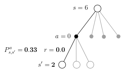
Environment transition probabilities and rewards are stored in array env.env.P. For example, if agent is in state 6 and select action 'West' (action 0), then env.env.P[6][0] stores all possible transitions from that state-action pair to next-states along with expected rewards.
env.env.P[6][0]
Above tells us, that after selectin action 'West', wind can blow us to three possible states:
- given starting state 6 and action 0 (West), there is 0.33 chance ending in state 2, with reward 0.0, non-terminal
- given starting state 6 and action 0 (West), there is 0.33 chance ending in state 5, with reward 0.0, terminal (hole)
- given starting state 6 and action 0 (West), there is 0.33 chance ending in state 10, with reward 0.0, non-terminal
Perhaps this is better ilustrated with a diagram
Perhaps good time to introduce notation:
- Probabilities
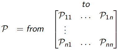
- $\mathbf{P}^\pi$ - transition probability matrix under our policy $\pi$ with shape [nb_states, nb_states]
- $P_{s,s'}^\pi$ - transition probability from state s to s' under current policy $\pi$, these are elements of matrix $\mathbf{P}^\pi$
- $P_{s,s'}^a$ - transition probability from state-action s,a to state s' (this is 33% above)
- $\pi(a|s)$ - policy - probability of choosing action a, given state s - defined by us
- Expected Rewards
- $\mathbf{R}^\pi$ is vector of expected rewards for each state
- $R_s^\pi$ - expected reward on transition from state s to any state s' (weighted sum over all actions), these are elements of vector $\mathbf{R}^\pi$
- $R_s^a$ - expected reward on transition from state-action s,a to any next state (weighted sum over all next-states)
- $R_{s,s'}^a$ - expected reward on transition from state-action s,a to state s' (this is 0.0 above)
- State Values
- $\mathbf{v}^{k+1}$ is vector of state-values $v(s)$ at iteration k+1
- $\mathbf{v}^k$ is vector of state-values $v(s)$ at iteration k
- $\gamma$ is a discount factor, here equals 1.0
Iterative Policy Evaluation
Policy Evaluation can be implemented in two ways:
- Iterate over every state s and perform backup using Bellman Expectation Equation
- Calculate matrix $\mathbf{P}^\pi$ and vector $\mathbf{R}^\pi$ and perform backup in matrix form
Because we evaluate fixed policy matrix $\mathbf{P}^\pi$ and vector $\mathbf{R}^\pi$ are constant. They need to be computed only once, then we can do backup over and over again in matrix form.
We will implement following algorithm to evaluate our fixed random policy:
- Flatten Markov Decision Process to Markov Reward Process, i.e. assume policy is part of environment
- Initialize all state values to zero: $\mathbf{v \leftarrow 0}$
- Iterate k=100 times:
- update all state values using Bellman Expectation Equation:
$$ \Large{ \mathbf{v}^{k+1} = \mathbf{R}^\pi + \gamma \mathbf{P}^\pi \mathbf{v}^k } $$
First we will calculate transition probability from state s to s' as follows
$$ \Large{ P^\pi_{s,s'}=\sum_{a \in A} \pi(a|s) P^a_{s,s'} } $$
Then we use $P_{s,s'}^\pi$ to form transition probability matrix $\mathbf{P}^\pi$
Second we calculate expected reward on transition from state-action pair
$$ \Large{ R^a_s = \sum_{s' \in S} P^a_{s,s'} R^a_{s,s'} } $$
Now we can calculate expected reward from state s (not state-action!) to any next state
$$ \Large{ R^\pi_s = \sum_{a \in A} \pi(a|s) R^a_s } $$
Helper function to calculate both $\mathbf{P}^\pi$ and $\mathbf{R}^\pi$
def flatten_mdp(policy, model):
    P_pi = np.zeros([nb_states, nb_states])  # transition probability matrix (s) to (s')
    R_pi = np.zeros([nb_states])             # exp. reward from state (s) to any next state
    for s in range(nb_states):
        for a in range(nb_actions):
            for p_, s_, r_, _ in model[s][a]:
                # p_ - transition probability from (s,a) to (s')
                # s_ - next state (s')
                # r_ - reward on transition from (s,a) to (s')
                P_pi[s, s_] += policy[s,a] * p_   # transition probability (s) -> (s')
                Rsa = p_ * r_                     # exp. reward from (s,a) to any next state
                R_pi[s] += policy[s,a] * Rsa      # exp. reward from (s) to any next state
    assert np.alltrue(np.sum(P_pi, axis=-1)==np.ones([nb_states]))  # rows should sum to 1
    return P_pi, R_pi
Let's do policy evaluation for random policy
policy = np.ones([nb_states, nb_actions]) / nb_actions  # 0.25 probability for each action
P_pi, R_pi = flatten_mdp(policy, model=env.env.P)
print(P_pi)
print(R_pi)
Perform 100 steps of iterative policy evaluation according to equation
$$ \Large{ \mathbf{v}^{k+1} = \mathbf{R}^\pi + \gamma \mathbf{P}^\pi \mathbf{v}^k } $$
lmbda = 1.0  # discount

V_pi = np.zeros([nb_states])
for k in range(100):
    V_pi = R_pi + lmbda * P_pi @ V_pi
print(V_pi.reshape([4, -1]).round(3))
Correct output:
[[0.014 0.012 0.021 0.01 ]
 [0.016 0.    0.041 0.   ]
 [0.035 0.088 0.142 0.   ]
[0. 0.176 0.439 0. ]]Policy Iteration
We will implement following algorithm:
- repeat n=10 times:
- flatten current policy into MRP
- perform k=100 steps of Policy Evaluation
- perform greedy policy improvement (requires q values)
To do policy improvement we need to know best action, which means we need to calculate action-values for all state-action pairs. Diagram below shows how to calculate action-values using Bellman Expectation Equation
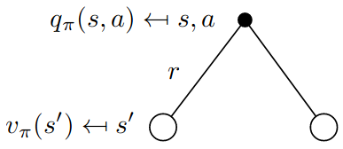
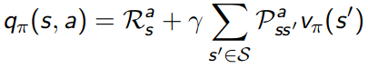
Helper function to calculate vector $\mathbf{Q^\pi}$ of action-values for all actions, each elements is corresponding $q_\pi(s,a)$
def calc_Q_pi(V_pi, model, lmbda):
    Q_pi=np.zeros([nb_states, nb_actions])
    for s in range(nb_states):
        for a in range(nb_actions):
            for p_, s_, r_, _ in model[s][a]:
                # p_ - transition probability from (s,a) to (s')
                # s_ - next state (s')
                # r_ - reward on transition from (s,a) to (s')
                Rsa = p_ * r_   # expected reward for transition s,a -> s_
                Vs_ = V_pi[s_]  # state-value of s_
                Q_pi[s, a] += Rsa + lmbda * p_ * Vs_
    return Q_pi
Q_pi = calc_Q_pi(V_pi, env.env.P, lmbda)   # calc Q_pi for V_pi from previous section
print(Q_pi.round(3))
Correct output:
[[0.015 0.014 0.014 0.013]
 [0.009 0.012 0.011 0.016]
 [0.024 0.021 0.024 0.014]
 [0.01  0.01  0.007 0.014]
 [0.022 0.017 0.016 0.01 ]
 [0.    0.    0.    0.   ]
 [0.054 0.047 0.054 0.007]
 [0.    0.    0.    0.   ]
 [0.017 0.041 0.035 0.046]
 [0.07  0.118 0.106 0.059]
 [0.189 0.176 0.16  0.043]
 [0.    0.    0.    0.   ]
 [0.    0.    0.    0.   ]
 [0.088 0.205 0.234 0.176]
 [0.252 0.538 0.527 0.439]
[0. 0. 0. 0. ]]Actual Policy Iteration algorithm. Start with random policy
V_pi = np.zeros([nb_states])
policy = np.ones([nb_states, nb_actions]) / nb_actions  # random policy, 25% each action
lmbda = 1.0  # discount

for n in range(10):
    # flatten MDP
    P_pi, R_pi = flatten_mdp(policy, env.env.P)

    # evaluate policy
    for k in range(100):
        V_pi = R_pi + lmbda * P_pi @ V_pi

    # iterate policy
    Q_pi = calc_Q_pi(V_pi, env.env.P, lmbda)
    a_max = np.argmax(Q_pi, axis=-1)     # could distribute actions between all max(q) values
    policy *= 0  # clear
    policy[range(nb_states), a_max] = 1  # pick greedy action
Show optimal policy
a2w = {0:'<', 1:'v', 2:'>', 3:'^'}
policy_arrows = [a2w[x] for x in np.argmax(policy, axis=-1)]
print(np.array(policy_arrows).reshape([-1, 4]))
Correct optimal policy:
[['<' '^' '^' '^']
 ['<' '<' '<' '<']
 ['^' 'v' '<' '<']
['<' '>' 'v' '<']]Value Iteration
Similarly to Policy Evaluation, backup can be performed in matrix form, or by iterating over states. Because state-values change every step, I think it is more intuitive to perform Value Iteration by iterating over states (this is what calc_Q_pi does).
Algorithm:
- Iterate n=50 times:
- perform Bellman Optimality Equation backup
For reference
$$ \Large{ v_{k+1}(s) = \max\limits_{a \in A} q_k(s,a) } $$
V_pi = np.zeros([nb_states])
lmbda = 1.0 # discount
for n in range(50):
Q_pi = calc_Q_pi(V_pi, env.env.P, lmbda)
a_max = np.argmax(Q_pi, axis=-1)
V_pi = Q_pi[range(nb_states), a_max]
# construct policy
policy = np.zeros([nb_states, nb_actions])
policy[range(nb_states), a_max] = 1
Show optimal policy
a2w = {0:'<', 1:'v', 2:'>', 3:'^'}
policy_arrows = [a2w[x] for x in np.argmax(policy, axis=-1)]
print(np.array(policy_arrows).reshape([-1, 4]))
Correct optimal policy:
[['<' '^' '^' '^']
 ['<' '<' '<' '<']
 ['^' 'v' '<' '<']
 ['<' '>' 'v' '<']]