$$ \huge{\underline{\textbf{ Model Free Control - Off Policy }}} $$
$$ \Large{\textbf{ Part 2: Expectation Based Methods }} $$
Contents
Intro
- Sources
- Introduction
- Imports - import stuff from part 1
- SARSA - Refresher - refresher from part 1
Expectation Based Methods
- Q-Learning
- Expected SARSA - off-policy version of standard SARSA using expectations
- Tree Backup - multi-step Expected SARSA
Sources
- UCL Course on RL: http://www0.cs.ucl.ac.uk/staff/d.silver/web/Teaching.html
- Lecture 5 pdf: http://www0.cs.ucl.ac.uk/staff/d.silver/web/Teaching_files/control.pdf
- Lecture 5 vid: https://www.youtube.com/watch?v=0g4j2k_Ggc4
- Sutton and Barto 2018: http://incompleteideas.net/book/the-book-2nd.html
Introduction
This post roughly corresponds to part 2 of Lecture 5 of UCL RL course by David Silver.
We will explore off-policy algorithms as per videos. In this part we focus on Q-Learning and expectation based algorithms. In next part we deal with importance sampling. In addition to Q-Learning we will look into Expected SARSA (1-step off-policy) and Tree Backup (n-step off-policy) algorithms.
As terminology can be a bit confusing, let's have a quick look at our little zoo of RL algorithms

To better explain differences between On-Policy, Expectation and Importance Sampling, let's consider a mini-MDP below
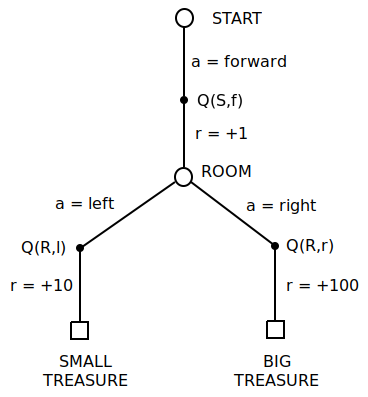
- agent starts in state START, then automatically picks action forward (no choice here)
- after going forward, agent finds a gold coin (+1 reward) and ends up in a state ROOM
- from the ROOM, agent can go either left or right with probability determined by policy under consideration
- if agent goes left, then it ends up finding SMALL TREASURE (+10 reward), MDP terminates
- if agent goes right, then it finds LARGE TREASURE (+100 reward), MDP terminates
- mini-MDP is fully deterministic
Let's consider state-action values in reverse order:
- Assume all Q-values are initialised to zero
- Assume no discounting
- $Q(ROOM,left)$ or $Q(R,l)$ - as long as it is being explored, it will evaluate to correct value +10, and it doesn't depend on policy, this isn't very interesting
- $Q(ROOM,right)$ or $Q(R,r)$ - same as above
- $Q(START,forward)$ or $Q(S,f)$ - this one we are interested in. It very much depends on policy being executed, for example for random policy
$$ Q(S,f) = 1 + .5*Q(R,l) + .5*Q(R,r) = 1 + 5 + 50 = 56 $$
For each algorithm we will show different ways we can backup
$$ Q(S,f) \leftarrow Q(R,l), Q(R,r) $$
But first let's get some setup code out of the way
Imports
import numpy as np
import matplotlib.pyplot as plt
Environment is exactly the same as in previous post

from ModelFreeControl_Part1 import LinearEnv, REF_RANDOM, REF_GREEDY
Let's create environment and policies for future use
env = LinearEnv()

pi_random = np.tile([0.50, 0.50], [11, 1])  # starting random policy
pi_greedy = np.tile([0.00, 1.00], [11, 1])  # optimal greedy policy
pi_skewed = np.tile([0.40, 0.60], [11, 1])  # will use this later
And import common functions, they are also exactly the same as in previous post
from ModelFreeControl_Part1 import generate_episode, LogEntry, plot_experiments
SARSA - Refresher
Puropose of this section is to show how good old SARSA works on our mini-MDP. Show problems with on-policy exploration, and then in subsequent sections we will show how Q-Learning, Expected SARSA and Importance Sampling solve these problems.
Code for SARSA was introduced in previous post. I repeat it here for convenience. We will treat SARSA, N-Step SARSA and MC Control as together. The main difference between them is backup length. Other than that, the underlying principle is the same:
- update Q-value estimation
- update policy towards $\epsilon$-greedy
SARSA update formula
$$ Q(S_t,A_t) \leftarrow Q(S_t,A_t) + \alpha \big[ \color{blue}{R_{t+1} + \gamma Q(S_{t+1},A_{t+1}) }\color{black}{} - Q(S_t,A_t) \big] $$
How does SARSA update $Q(S,f)$? By repeated sampling, for example for random policy sometimes we backup from $Q(R,l)$, sometimes from $Q(R,r)$. Becouse we update only a little bit (this is by $\alpha$) towards each target every time, value eventually settles on weighted average between $Q(R,l)$ and $Q(R,r)$ plus reward +1.
That is all nice and rosy as long as actually keep visiting all states. If policy is greedy, and it locks itself into always choosing left action before properly evaluating $Q(R,r)$ then agent is doomed, it will never discover big treasure.
This demonstrates the main problem with on-policy methods. We have to use $\epsilon$-greedy policy to guarantee continuous exploration. But when we use $\epsilon$-greedy agent will not achieve optimal performance. We could decay $\epsilon$ with time, but that brings practical issues with establishing correct schedule.
Let's import SARSA code from previous post and repeat the experiment.
from ModelFreeControl_Part1 import make_eps_greedy, mc_control, sarsa
log = []
for _ in range(5):
    hist, perf = sarsa(env, pi_random, N=200, alpha=0.1, eps=0.1)
    log.append(LogEntry('sarsa', hist, perf))
plot_experiments(log, REF_GREEDY, 'SARSA')

Note on Exploring Starts
We could guarantee continuous exploration by starting episode at random state and with random first action every time and then following given policy. This would guarantee all state-action pairs are evaluated, and subsequently fix the problem we encountered above. After whole MDP is correctly evaluated we can switch off exploring starts and operate as normal in now solved MDP. This works disregarding if policy is greedy or not.
Problem with this is that it only works in small state spaces and usually can't be applied in real-world scenarios (how do you teleport robot into random initial states?).
Imagine yourself you are a wizard on a journey to find treasure. Tomorrow you will be allowed to enter mini-MDP for exactly one attempt to collect as much gold as possible. There will be no repeats. But being clever and powerful wizard, you figured out you can enter mini-MDP today in a ghost form, you won't be able collect gold today, but you can explore mini-MDP and prepare yourself for tomorrow. Actually you can enter it in a ghost form as many times as you want.
You want to make sure you explore all possible routes, so you follow random policy. But you are interested in maximum possible gold you can gather. So every time you visit a state-action pair you write down maximum possible gold you can collect from there onwards. After couple trials you note down values for $Q(R,l)$ and $Q(R,r)$ to be +10 and +100 respectively. Now you wonder what is max possible gold from $Q(S,f)$? Well, that is +1 gold coin, and then +100, because obviously on the actual trial tomorrow you will pick right door. So your backup looks like this
$$ Q(S,f) \leftarrow Q(S,f) + \alpha \big[ \color{blue}{R + \gamma \max[Q(R,l), Q(R,r)]} \color{black}{} - Q(S,f) \big] $$
Or more generally
$$ Q(S_t,A_t) \leftarrow Q(S_t,A_t) + \alpha \big[ \color{blue}{R_{t+1} + \gamma \max\limits_{a' \in A} Q(S_{t+1},a') }\color{black}{} - Q(S_t,A_t) \big] $$
Taa daa, and this is famous Q-Learning. Note that even if you had more choices form START state, then you know you can always get +101 reward by following action forward. Mini-MDP could be deeper, have more branches etc. same rules apply. If mini-MDP was nondeterministic, then you need to sample multiple times per action-value to properly estimate reward and environment dynamics, but other than that everything stays the same.
Let's modify SARSA as follows:
- introduce behavioural policy along target policy
- remove eps parameter
- roll two trajectories from each episode:
- one as before
- one to evaluate target policy, so we can plot agent progress
- modify target line with new update rule
- update target policy always towards greedy
- evaluate performance based on target policy
def q_learning(env, pol_beh, pol_tar, N, alpha):
    hist, perf = [], []
    Q = np.zeros(shape=[env.nb_st, env.nb_act])
    for ep in range(N):
        trajectory = generate_episode(env, pol_beh)
        trajectory_2 = generate_episode(env, pol_tar)
        for t in range(len(trajectory)-1):
            St, _, _, At = trajectory[t]
            St_1, Rt_1, _, At_1 = trajectory[t+1]
            # target = Rt_1 + 1.0 * Q[St_1, At_1]  # SARSA
            target = Rt_1 + 1.0 * np.max(Q[St_1,:])  # Q-Learning
            Q[St, At] = Q[St, At] + alpha * (target - Q[St, At])

        pol_tar = make_eps_greedy(Q, eps=0.0)  # eps always 0.0 to make policy greedy

        hist.append(Q.copy())
        perf.append(len(trajectory_2)-1)
    return np.array(hist), np.array(perf)
log = []
for _ in range(5):
    hist, perf = q_learning(env, pi_random, pi_random, N=200, alpha=0.1)
    log.append(LogEntry('q_learning', hist, perf))
plot_experiments(log, REF_GREEDY, 'Q-Learning')

Woo, perfect performance.
In example above we keep behavioural policy random through whole learning process. Nothing stops us from improving behavioural policy as well. We could, for example follow $\epsilon$-greedy policy as behavioural - keep improving it towards "good" choices, but still allow for exploration. Actually, in most case we would not have explicit "policy" table, we would pick actions on the fly according to current Q-Values.
Expected SARSA
Let's assume we are performing SARSA updates while following random policy. Let's also assume $Q(R,l)$ and $Q(R,r)$ have been correctly evaluated already. There is alternative way to backup $Q(S,f)$ from $Q(R,l)$ and $Q(R,r)$. Namely we know what policy we are following. We know we will pick $Q(R,l)$ 50% of a time and $Q(R,r)$ 50% of a time. Then why not backup towards weighted average stright away?
$$ Q(S,f) \leftarrow Q(S,f) + \alpha \big[ \color{blue}{R + \gamma\pi(l|R)Q(R,l)+\gamma\pi(r|R)Q(R,r)} \color{black}{} - Q(S,f) \big] $$
Or more generally
$$ Q(S_t,A_t) \leftarrow Q(S_t,A_t) + \alpha \big[ \color{blue}{R_{t+1} + \gamma \sum_{a' \in A} \pi(a'|S_{t+1})Q(S_{t+1},a') }\color{black}{} - Q(S_t,A_t) \big] $$
Of course we still need to sample to learn about rewards at each time-step.
Now what if we want to follow one policy, and evaluate another one?
Going back to wizard example, let's assume different task, let's say oracle asks you to evaluate random policy, but you can always only follow skewed policy 40%/60% left/right (oracle knows if you cheat). You figure as follows:
- $Q(R,l)$ and $Q(R,r)$ will evaluate correctly to +10 and +100 no matter what is behavioural and target policy (as long as you keep visiting them)
- as per $Q(S,f)$, you know that under target policy, you will visit $Q(R,l)$ 50% of a time and $Q(R,r)$ 50% of time, so you can do backup as per equations above, just plug in target policy and you get correct $Q(S,f)$ for target policy. Actually behavioural policy doesn't matter, as long as it keeps visiting $Q(S,f)$
- above hold true no matter how many levels deep you go, or even if MDP is loopy
Let's write some code, changes from q_learning are as follows:
- introduce learn param, so we can disable policy improvement for now
- change target line with new update equation
def exp_sarsa(env, pol_beh, pol_tar, N, alpha, learn=True):
    hist, perf = [], []
    Q = np.zeros(shape=[env.nb_st, env.nb_act])
    for ep in range(N):
        trajectory = generate_episode(env, pol_beh)
        trajectory_2 = generate_episode(env, pol_tar)
        for t in range(len(trajectory)-1):
            St, _, _, At = trajectory[t]
            St_1, Rt_1, _, At_1 = trajectory[t+1]
            # target = Rt_1 + 1.0 * Q[St_1, At_1]  # SARSA
            # target = Rt_1 + 1.0 * (pol_tar[St_1, 0]*Q[St_1, 0] + pol_tar[St_1, 1]*Q[St_1, 1])  # exp sarsa
            target = Rt_1 + 1.0 * np.sum(pol_tar[St_1,:] * Q[St_1,:]) # exp sarsa, equivalent to above
            Q[St, At] = Q[St, At] + alpha * (target - Q[St, At])

        if learn:  # set eps to None to disable improvement step
            pol_tar = make_eps_greedy(Q, 0.0)  # eps 0.0 makes policy greedy

        hist.append(Q.copy())
        perf.append(len(trajectory_2)-1)
    return np.array(hist), np.array(perf)
Off-Policy Prediction
Skewed behavioural policy, as per oracle task.
pi_skewed = np.tile([0.40, 0.60], [11, 1]) # go right a bit more often
And evaluate random policy while following skewed policy. With Expected SARSA we can set alpha to much higher value. Actually, because our MDP is fully deterministic, we can safely set it all the way to 1.0.
log = []
for _ in range(5):
    hist, perf = exp_sarsa(env, pi_skewed, pi_random, N=200, alpha=1.0, learn=False)
    log.append(LogEntry('follow-skew-eval-rand', hist, perf))
plot_experiments(log, REF_RANDOM, 'Expected SARSA - Follow Skewed, Eval Random')

Notice low variance. Even though we are following skewed policy, expectation based backups converge much quicker than equivalent sample based backups. Compare this with TD Prediction from previous part
Off-Policy Control
Enable learning. With greedy target policy (eps internally set to zero) this is equivalent to Q-Learning
log = []
for _ in range(5):
    hist, perf = exp_sarsa(env, pi_random, pi_random, N=200, alpha=1.0, learn=True)
    log.append(LogEntry('exp-sarsa', hist, perf))
plot_experiments(log, REF_GREEDY, 'Expected SARSA Control')

Tree Backup
There are two n-step extensions to Expected SARSA: N-Step Expected SARSA (on-policy) and Tree Backup (off-policy). Here we only describe Tree Backup
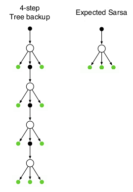
Above is a quick comparison of Expected SARSA and Tree Backup. Nodes over which we calculate expectations are marked in green. In Tree Backup we use expectation at every time step. You can use fixed number of steps (e.g. nstep=5) or follow full trajectory (nstep=inf).
For more details, see Sutton and Barto (2018), chapter 7.5 "Off-policy Learning Without Importance Sampling: The n-step Tree Backup Algorithm".
Note that this is not exact replica of algorithm in the book. Most important differences:
- this version only works with discount 1.0
- this version is offline, book version is online
def tree_backup(env, pol_beh, pol_tar, N, alpha, nstep=float('inf'), learn=True):
    hist, perf = [], []
    Q = np.zeros(shape=[env.nb_st, env.nb_act])
    for ep in range(N):
        trajectory = generate_episode(env, pol_beh)
        trajectory_2 = generate_episode(env, pol_tar)
        for t in range(len(trajectory)-1):
            St, _, _, At = trajectory[t]

            disc = 1.0              # discount, tested with disc==1.0 only!
            T = len(trajectory)-1   # terminal state
            max_j = min(t+nstep, T) # last state iterated, inclusive
            tmp_disc = 1.0          # this will decay
            pol_mult = 1.0
            target = 0
            # weights = 0  # debug

            # Iterate from t+1 to t+nstep or T (inclusive start and finish)
            for j in range(t+1, max_j+1):
                Sj, Rj, _, Aj = trajectory[j]
                if j != max_j:
                    # not-last-step, backup all Act != At
                    target += tmp_disc * pol_mult * (Rj + disc * (np.sum(pol_tar[Sj,:] * Q[Sj,:]) \
                                                                  - pol_tar[Sj,Aj] * Q[Sj,Aj]))
                    # weights += pol_mult * (np.sum(pol_tar[Sj,:]) - pol_tar[Sj,Aj])  # debug
                else:
                    # last step, backup all
                    target += tmp_disc * pol_mult * (Rj + disc * np.sum(pol_tar[Sj,:] * Q[Sj,:]))
                    # weights += pol_mult * np.sum(pol_tar[Sj,:])  # debug
                tmp_disc *= disc
                pol_mult *= pol_tar[Sj, Aj]
            # assert weights == 1  # debug

            Q[St, At] = Q[St, At] + alpha * (target - Q[St, At])

        if learn:  # set eps to None to disable improvement step
            pol_tar = make_eps_greedy(Q, 0.0)  # eps 0.0 makes policy greedy

        hist.append(Q.copy())
        perf.append(len(trajectory_2)-1)
    return np.array(hist), np.array(perf)
Off-Policy Prediction
Evaluate random policy while following skewed policy. With nstep set to "1" Tree Backup is equivalent to Expected Sarsa
log = []
for _ in range(5):
    # hist, perf = tree_backup(env, pi_skewed, pi_random, N=200, alpha=1, nstep=1, learn=False)
    hist, perf = tree_backup(env, pi_skewed, pi_random, N=200, alpha=1, nstep=5, learn=False)
    log.append(LogEntry('tree-backup', hist, perf))
plot_experiments(log, REF_RANDOM, 'Tree Backup - Follow Skewed, Eval. Random')

Off-Policy Control
Improve target policy to be greedy. Perhaps we could call this N-Step Q-Learning?
Note that if target policy is greedy, then algorithm will backup steps up to a point where greedy policy diverges from actual steps taken.
log = []
for _ in range(5):
    hist, perf = tree_backup(env, pi_skewed, pi_random, N=200, alpha=1, nstep=5, learn=True)
    log.append(LogEntry('tree-backup', hist, perf))
plot_experiments(log, REF_GREEDY, 'Tree Backup Control')
