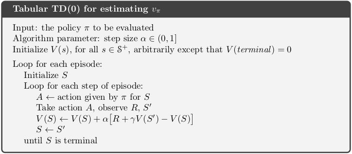
$$ \huge{\underline{\textbf{ TD Prediction }}} $$
def td_prediction(env, policy, ep, gamma, alpha):
    """TD Prediction

    Params:
        env - environment
        ep - number of episodes to run
        policy - function in form: policy(state) -> action
        gamma - discount factor [0..1]
        alpha - step size (0..1]
    """
    assert 0 < alpha <= 1
    V = defaultdict(float)    # default value 0 for all states

    for _ in range(ep):
        S = env.reset()
        while True:
            A = policy(S)
            S_, R, done = env.step(A)
            V[S] = V[S] + alpha * (R + gamma * V[S_] - V[S])
            S = S_
            if done: break

    return V
For TD prediction to work, V for terminal states must be equal to zero, always. Value of terminal states is zero because game is over and there is no more reward to get. Value of next-to-last state is reward for last transition only, and so on.
- If terminal state is initalised to something different than zero, then your resulting V estimates will be offset by that much
- If, God forbid, V of terminal state is updated during training then everything will go monkey balls.
- so make absolutely sure environment returns different observations for terminal states than non-terminal ones
- hint: this is not the case for gym Blackjack
 |
 |
Evaluate Example 6.2
This environment is defined further in the book, but is very simple and useful here.
import numpy as np
import matplotlib.pyplot as plt
from mpl_toolkits.mplot3d import axes3d
from collections import defaultdict
import gym  # blacjack
Define and create environment. See Sutton and Barto (2018) Example 6.2
class LinearEnv:
    """
    State Index:   [ 0    1    2    3    4    5    6 ]
    State Label:   [ .    A    B    C    D    E    . ]
    Type:          [ T    .    .    S    .    .    T ]
    """
    V_true =       [0.0, 1/6, 2/6, 3/6, 4/6, 5/6, 0.0]

    def __init__(self):
        self.reset()

    def reset(self):
        self._state = 3
        self._done = False
        return self._state

    def step(self, action):
        if self._done: raise ValueError('Episode has terminated')
        if action not in [0, 1]: raise ValueError('Invalid action')

        if action == 0: self._state -= 1
        if action == 1: self._state += 1

        reward = 0
        if self._state < 1: self._done = True
        if self._state > 5: self._done = True; reward = 1

        return self._state, reward, self._done  # obs, rew, done
env = LinearEnv()
Plotting function
def plot(V_dict):
    """Param V is dictionary int[0..7]->float"""

    V_arr = np.zeros(7)
    for st in range(7):
        V_arr[st] = V_dict[st]

    fig = plt.figure()
    ax = fig.add_subplot(111)
    ax.plot(LinearEnv.V_true[1:-1], color='black', label='V true')
    ax.plot(V_arr[1:-1], label='V')

    ax.legend()

    plt.show()
Random policy
def policy(state):
    return np.random.choice([0, 1])  # random policy
Solve environment.
- Note that we initialise V with 0 here, in the book V is initialised to 0.5 for non-terminal states, see further below for example with V_init=0.5
V = td_prediction(env, policy, ep=1000, gamma=1.0, alpha=0.1)
plot(V)

Evaluate Blackjack
See Example 5.1 for details. Evaluate naive policy (stick on 20 or more, hit otherwise) on blackjack. This correponds to similar evaluation we have done with First Visit MC Prediction algorithm in chapter 5.1.
As mentioned earlier, there is a problem with Blackjack environment in the gym. If agent sticks, then environment will return exactly the same observation but this time with done==True. This will cause TD prediction to evaluate terminal state to non-zero value belonging to non-terminal state with same observation. We fix this by redefining observation for terminal states with 'TERMINAL'.
class BlackjackFixed():
    def __init__(self):
        self._env = gym.make('Blackjack-v0')

    def reset(self):
        return self._env.reset()

    def step(self, action):
        obs, rew, done, _ = self._env.step(action)
        if done:
            return 'TERMINAL', rew, True  # (obs, rew, done)         <-- SUPER IMPORTANT
        else:
            return obs, rew, done
        return self._env.step(action)
env = BlackjackFixed()
Naive policy for blackjack
def policy(St):
    p_sum, d_card, p_ace = St
    if p_sum >= 20:
        return 0  # stick
    else:
        return 1  # hit
Plotting
def plot_blackjack(V_dict):
    def convert_to_arr(V_dict, has_ace):
        V_dict = defaultdict(float, V_dict)  # assume zero if no key
        V_arr = np.zeros([10, 10])  # Need zero-indexed array for plotting
        for ps in range(12, 22):     # convert player sum from 12-21 to 0-9
            for dc in range(1, 11):  # convert dealer card from 1-10 to 0-9
                V_arr[ps-12, dc-1] = V_dict[(ps, dc, has_ace)]
        return V_arr

    def plot_3d_wireframe(axis, V_dict, has_ace):
        Z = convert_to_arr(V_dict, has_ace)
        dealer_card = list(range(1, 11))
        player_points = list(range(12, 22))
        X, Y = np.meshgrid(dealer_card, player_points)
        axis.plot_wireframe(X, Y, Z)

    fig = plt.figure(figsize=[16,3])
    ax_no_ace = fig.add_subplot(121, projection='3d', title='No Ace')
    ax_has_ace = fig.add_subplot(122, projection='3d', title='With Ace')
    ax_no_ace.set_xlabel('Dealer Showing'); ax_no_ace.set_ylabel('Player Sum')
    ax_has_ace.set_xlabel('Dealer Showing'); ax_has_ace.set_ylabel('Player Sum')
    plot_3d_wireframe(ax_no_ace, V_dict, has_ace=False)
    plot_3d_wireframe(ax_has_ace, V_dict, has_ace=True)
    plt.show()
Evaluate
V = td_prediction(env, policy, ep=50000, gamma=1.0, alpha=0.05)
plot_blackjack(V)

Recreate Example 6.2 figures
We will need slightly extended version of TD prediction, so we can log V during training and initalise V to 0.5
def td_prediction_ext(env, policy, ep, gamma, alpha, V_init=None):
    """TD Prediction

    Params:
        env - environment
        ep - number of episodes to run
        policy - function in form: policy(state) -> action
        gamma - discount factor [0..1]
        alpha - step size (0..1]
    """
    assert 0 < alpha <= 1

    # Change #1, allow initialisation to arbitrary values
    if V_init is not None:  V = V_init.copy()       # remember V of terminal states must be 0 !!
    else:                   V = defaultdict(float)  # default value 0 for all states

    V_hist = []

    for _ in range(ep):
        S = env.reset()
        while True:
            A = policy(S)
            S_, R, done = env.step(A)
            V[S] = V[S] + alpha * (R + gamma * V[S_] - V[S])
            S = S_
            if done: break

        V_arr = [V[i] for i in range(7)]  # e.g. [0.0, 0.3, 0.4, 0.5, 0.6. 0.7, 0.0]
        V_hist.append(V_arr)  # dims: [ep_number, state]

    return V, np.array(V_hist)
Environment and policy
env = LinearEnv()
def policy(state):
    return np.random.choice([0, 1])  # random policy
Left figure
V_init = defaultdict(lambda: 0.5)   # init V to 0.5
V_init[0] = V_init[6] = 0.0         # but terminal states to zero !!
V_n1, _ = td_prediction_ext(env, policy, ep=1, gamma=1.0, alpha=0.1, V_init=V_init)
V_n10, _ = td_prediction_ext(env, policy, ep=10, gamma=1.0, alpha=0.1, V_init=V_init)
V_n100, _ = td_prediction_ext(env, policy, ep=100, gamma=1.0, alpha=0.1, V_init=V_init)

def to_arr(V_dict):
    """Param V is dictionary int[0..7]->float"""
    V_arr = np.zeros(7)
    for st in range(7):
        V_arr[st] = V_dict[st]
    return V_arr

V_n1 = to_arr(V_n1)
V_n10 = to_arr(V_n10)
V_n100 = to_arr(V_n100)

fig = plt.figure()
ax = fig.add_subplot(111)
ax.plot(np.zeros([7])[1:-1]+0.5, color='black', linewidth=0.5)
ax.plot(LinearEnv.V_true[1:-1], color='black', label='True Value')
ax.plot(V_n1[1:-1], color='red', label='n = 1')
ax.plot(V_n10[1:-1], color='green', label='n = 10')
ax.plot(V_n100[1:-1], color='blue', label='n = 100')
ax.set_title('Estimated Value')
ax.set_xlabel('State')
ax.legend()

# plt.savefig('assets/fig_0601a')
plt.show()

Right figure
Right figure is comparison between TD Prediction and Running Mean MC Prediction, so first thing we need is to define running mean MC algorithm. This code is adaptation of First Visit MC Prediction we did earlier. See book chapter 5.1.
def mc_prediction_ext(env, policy, ep, gamma, alpha, V_init=None):
    """Running Mean MC Prediction
    Params:
        env - environment
        policy - function in a form: policy(state)->action
        ep - number of episodes to run
        gamma - discount factor [0..1]
        alpha - step size (0..1)
        V_init - inial V
    """
    if V_init is not None:  V = V_init.copy()
    else:                   V = defaultdict(float)  # default value 0 for all states

    V_hist = []

    for _ in range(ep):
        traj, T = generate_episode(env, policy)
        G = 0
        for t in range(T-1,-1,-1):
            St, _, _, _ = traj[t]      # (st, rew, done, act)
            _, Rt_1, _, _ = traj[t+1]

            G = gamma * G + Rt_1

            V[St] = V[St] + alpha * (G - V[St])

        V_arr = [V[i] for i in range(7)]  # e.g. [0.0, 0.3, 0.4, 0.5, 0.6. 0.7, 0.0]
        V_hist.append(V_arr)  # dims: [ep_number, state]

    return V, np.array(V_hist)
def generate_episode(env, policy):
    """Generete one complete episode.

    Returns:
        trajectory: list of tuples [(st, rew, done, act), (...), (...)],
                    where St can be e.g tuple of ints or anything really
        T: index of terminal state, NOT length of trajectory
    """
    trajectory = []
    done = True
    while True:
        # === time step starts here ===
        if done:  St, Rt, done = env.reset(), None, False
        else:     St, Rt, done = env.step(At)
        At = policy(St)
        trajectory.append((St, Rt, done, At))
        if done:  break
        # === time step ends here ===
    return trajectory, len(trajectory)-1
For each line on a plot, we need to run algorithm multitple times and then calculate root-mean-squared-error over all runs properly. Let's define helper function to do all that.
def run_experiment(algorithm, nb_runs, env, ep, policy, gamma, alpha):
    V_init = defaultdict(lambda: 0.5)   # init V to 0.5
    V_init[0] = V_init[6] = 0.0         # but terminal states to zero !!

    V_runs = []
    for i in range(nb_runs):
        _, V_hist = algorithm(env, policy, ep, gamma=gamma, alpha=alpha, V_init=V_init)
        V_runs.append(V_hist)
    V_runs = np.array(V_runs)  # dims: [nb_runs, nb_episodes, nb_states=7]

    V_runs = V_runs[:,:,1:-1]  # remove data about terminal states (which is always zero anyway)
    error_to_true = V_runs - env.V_true[1:-1]
    squared_error = np.power(error_to_true, 2)
    mean_squared_error = np.average(squared_error, axis=-1)  # avg over states
    root_mean_squared_error = np.sqrt(mean_squared_error)
    rmse_avg_over_runs = np.average(root_mean_squared_error, axis=0)

    return rmse_avg_over_runs  # this is data that goes directly on the plot
And finally the experiments
#                                             nb_runs      ep         gamma alpha
rmse_td_a15 = run_experiment(td_prediction_ext, 100, env, 100, policy, 1.0, 0.15)
rmse_td_a10 = run_experiment(td_prediction_ext, 100, env, 100, policy, 1.0, 0.10)
rmse_td_a05 = run_experiment(td_prediction_ext, 100, env, 100, policy, 1.0, 0.05)
rmse_mc_a04 = run_experiment(mc_prediction_ext, 100, env, 100, policy, 1.0, 0.04)
rmse_mc_a03 = run_experiment(mc_prediction_ext, 100, env, 100, policy, 1.0, 0.03)
rmse_mc_a02 = run_experiment(mc_prediction_ext, 100, env, 100, policy, 1.0, 0.02)
rmse_mc_a01 = run_experiment(mc_prediction_ext, 100, env, 100, policy, 1.0, 0.01)
fig = plt.figure()
ax = fig.add_subplot(111)
ax.plot(rmse_mc_a04, color='red', linestyle='-', label='MC a=.04')
ax.plot(rmse_mc_a03, color='red', linestyle='--', label='MC a=.03')
ax.plot(rmse_mc_a02, color='red', linestyle=':', label='MC a=.02')
ax.plot(rmse_mc_a01, color='red', linestyle='-', label='MC a=.01')
ax.plot(rmse_td_a15, color='blue', linestyle='-', label='TD a=.15')
ax.plot(rmse_td_a10, color='blue', linestyle='--', label='TD a=.10')
ax.plot(rmse_td_a05, color='blue', linestyle=':', label='TD a=.05')
ax.set_title('Empirical RMS error, averaged over tests')
ax.set_xlabel('Walks / Episodes')
ax.legend()
plt.tight_layout()
# plt.savefig('assets/fig_0601b.png')
plt.show()
